Traffic sign recognition

This is the second project of self-driving cars engineer nanodegree. In this project we will recognize german traffic signs.

The goals / steps of this project are the following:

• Load the data set (see below for links to the project data set)
• Explore, summarize and visualize the data set
• Design, train and test a model architecture
• Use the model to make predictions on new images
• Analyze the softmax probabilities of the new images
• Summarize the results with a written report

Data Set Summary & Exploration

In this project, we use a german traffic sign dataset from German Dataset.

The code was tested on Google Colaboratory Platform. Check the Colaboratory Notebook.

1. Download the dataset:

import urllib.request

print('Beginning file download...')

url = 'https://s3-us-west-1.amazonaws.com/udacity-selfdrivingcar/traffic-signs-data.zip'

urllib.request.urlretrieve(url, './traffic-signs-data.zip')

2. Then, unzip the files in the root folder:

import zipfile
import os


print('Beginning file unzip')

zip_ref = zipfile.ZipFile('./traffic-signs-data.zip', 'r')
zip_ref.extractall('./')
zip_ref.close()

print('Done')
os.listdir("./")

3. The dataset is a pickled data. So, we use the next code to load the data

# Load pickled data
import pickle

# TODO: Fill this in based on where you saved the training and testing data

training_file = './train.p'
validation_file= './valid.p'
testing_file = './test.p'

with open(training_file, mode='rb') as f:
    train = pickle.load(f)
with open(validation_file, mode='rb') as f:
    valid = pickle.load(f)
with open(testing_file, mode='rb') as f:
    test = pickle.load(f)
    
X_train, y_train = train['features'], train['labels']
X_valid, y_valid = valid['features'], valid['labels']
X_test, y_test = test['features'], test['labels']

4. I used the pandas library to calculate summary statistics of the traffic signs data set:

import numpy as np
import pandas as pd

### Replace each question mark with the appropriate value. 
### Use python, pandas or numpy methods rather than hard coding the results

# TODO: Number of training examples
n_train = X_train.shape[0]

# TODO: Number of validation examples
n_validation = X_valid.shape[0]

# TODO: Number of testing examples.
n_test = X_test.shape[0]

# TODO: What's the shape of an traffic sign image?
image_shape = X_train.shape[1:]

# TODO: How many unique classes/labels there are in the dataset.
n_classes = len(np.unique(y_train))

print("Number of training examples =", n_train)
print("Number of testing examples =", n_test)
print("Number of validation examples =", n_validation)
print("Image data shape =", image_shape)
print("Number of classes =", n_classes)

After run the code I got these statistics:

• Number of training examples = 34799
• Number of testing examples = 12630
• Number of validation examples = 4410
• Image data shape = (32, 32, 3)
• Number of classes = 43

5. In the next to blocks of code, I define two methods show_images(images, cols = 1, titles = None) to show a group of images and select_random_images_by_classes(features, labels, n_features) which selects a random image for each class (43 clases) and then I use those methods to see how is structured the dataset visually.

def show_images(images, cols = 1, titles = None):
    """Display a list of images in a single figure with matplotlib.
    
    Parameters
    ---------
    images: List of np.arrays compatible with plt.imshow.
    
    cols (Default = 1): Number of columns in figure (number of rows is 
                        set to np.ceil(n_images/float(cols))).
    
    titles: List of titles corresponding to each image. Must have
            the same length as titles.
    """
    assert((titles is None)or (len(images) == len(titles)))
    
    n_images = len(images)
    
    if titles is None: titles = ['Image (%d)' % i for i in range(1,n_images + 1)]
    
    fig = plt.figure(figsize=(2, 2))
    
    for n, (image, title) in enumerate(zip(images, titles)):
        a = fig.add_subplot(cols, np.ceil(n_images/float(cols)), n + 1)
        a.grid(False)
        a.axis('off')
        if image.ndim == 2:
            plt.gray()
        plt.imshow(image, cmap='gray')
        a.set_title(title)
    
    fig.set_size_inches(np.array(fig.get_size_inches()) * n_images)
    plt.show()
    
def select_random_images_by_classes(features, labels, n_features):
  
  indexes = []
  _classes = np.unique(labels);
  
  while len(indexes) < len(_classes):
  
    index = random.randint(0, n_features-1)
    _class = labels[index]

    for i in range(0, len(_classes)):

      if _class == _classes[i]:
        _classes[i] = -1
        indexes.append(index)
        break

  images = []
  titles = []

  for i in range(0, len(indexes)):
    images.append(features[indexes[i]])
    titles.append("class " + str(labels[indexes[i]]))

  show_images(images, titles = titles)### Data exploration visualization code goes here.
### Feel free to use as many code cells as needed.
import matplotlib.pyplot as plt
import random
# Visualizations will be shown in the notebook.
%matplotlib inline

select_random_images_by_classes(X_train, y_train, n_train)

This code shows 43 random images (1 per class):

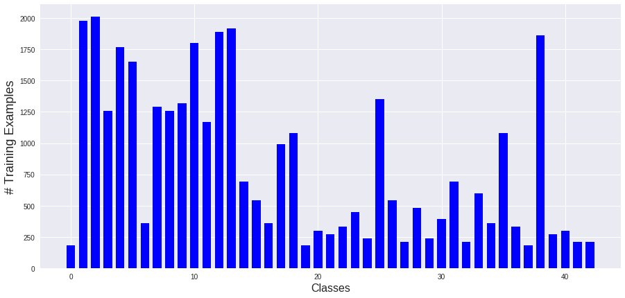
6. The next thing to do is to see how the dataset is distributed. So, I used the next two code blocks to see in a bar chart the # Training Data vs Classes:

def plot_distribution_chart(x, y, xlabel, ylabel, width, color):
  
  plt.figure(figsize=(15,7))
  plt.ylabel(ylabel, fontsize=18)
  plt.xlabel(xlabel, fontsize=16)
  plt.bar(x, y, width, color=color)
  plt.show()_classes, counts = np.unique(y_train, return_counts=True)

plot_distribution_chart(_classes, counts, 'Classes', '# Training Examples', 0.7, 'blue')

This will show the next chart:

7. This chart shows us that this dataset is poorly distributed. So, I use some Augmentation techniques to improve the dataset distribution.

import cv2

def augment_brightness_camera_images(image):
    image1 = cv2.cvtColor(image,cv2.COLOR_RGB2HSV)
    random_bright = .25+np.random.uniform()
    #print(random_bright)
    image1[:,:,2] = image1[:,:,2]*random_bright
    image1 = cv2.cvtColor(image1,cv2.COLOR_HSV2RGB)
    return image1

def transform_image(img,ang_range,shear_range,trans_range,brightness=0):
    '''
    This function transforms images to generate new images.
    The function takes in following arguments,
    1- Image
    2- ang_range: Range of angles for rotation
    3- shear_range: Range of values to apply affine transform to
    4- trans_range: Range of values to apply translations over.

    A Random uniform distribution is used to generate different parameters for transformation

    '''
    # Rotation

    ang_rot = np.random.uniform(ang_range)-ang_range/2
    rows,cols,ch = img.shape    
    Rot_M = cv2.getRotationMatrix2D((cols/2,rows/2),ang_rot,1)

    # Translation
    tr_x = trans_range*np.random.uniform()-trans_range/2
    tr_y = trans_range*np.random.uniform()-trans_range/2
    Trans_M = np.float32([[1,0,tr_x],[0,1,tr_y]])

    # Shear
    pts1 = np.float32([[5,5],[20,5],[5,20]])

    pt1 = 5+shear_range*np.random.uniform()-shear_range/2
    pt2 = 20+shear_range*np.random.uniform()-shear_range/2

    # Brightness

    pts2 = np.float32([[pt1,5],[pt2,pt1],[5,pt2]])

    shear_M = cv2.getAffineTransform(pts1,pts2)

    img = cv2.warpAffine(img,Rot_M,(cols,rows))
    img = cv2.warpAffine(img,Trans_M,(cols,rows))
    img = cv2.warpAffine(img,shear_M,(cols,rows))

    if brightness == 1:
      img = augment_brightness_camera_images(img)

    return img

This method get an image and apply some Rotation, Translation, Shear and Brightness transformations and then return it (Thanks to Vivek Yadav and his Image Augmentation repo).

Then, I tested the Augmentation method:

images = []

for i in range(0, 100):
  images.append(transform_image(X_train[555],10,5,5,brightness=1))

show_images(images)

So, from one image, we can create thousands of new images. This will make our dataset a more robust one.

for _class, count in zip(_classes, counts):
  new_images = []
  new_classes = []
  
  if count < 1000:
    y_train_length = y_train.shape[0]
    index = 0
    
    for i in range(0, 1000-count):
      while y_train[index] != _class:
        index = random.randint(0, y_train_length-1)
      new_images.append(transform_image(X_train[index],10,5,5,brightness=1))
      new_classes.append(_class)
      
    X_train = np.concatenate((X_train, np.array(new_images)))
    y_train = np.concatenate((y_train, np.array(new_classes)))
    
_classes, counts = np.unique(y_train, return_counts=True)

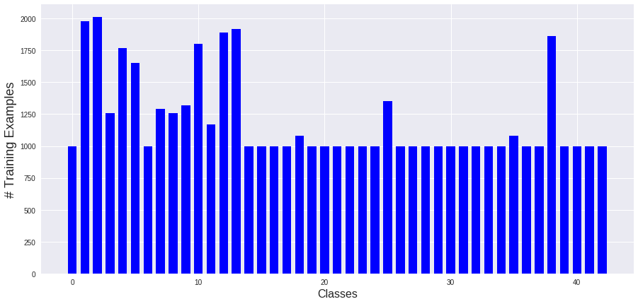
plot_distribution_chart(_classes, counts, 'Classes', '# Training Examples', 0.7, 'blue')

So, in the existing dataset, I look for classes that has less than 1,000 of examples, and for these classe I create 1000 - # Examples and add it to the dataset.

Now the dataset distribution has changed to this one:

Now we a more robust dataset!

#check dimentions

n_train = X_train.shape[0]

print("Number of training examples =", n_train)

The number of training examples has increased to 51690.

8. If we change the images to a grayscale ones, we could slightly improve the NN performance and easy change to make

X_train_gray = np.sum(X_train/3, axis=3, keepdims=True)

X_test_gray = np.sum(X_test/3, axis=3, keepdims=True)

X_valid_gray = np.sum(X_valid/3, axis=3, keepdims=True)

# check grayscale images
select_random_images_by_classes(X_train_gray.squeeze(), y_train, n_train)

9. According to CS231 class, for images is not strictly necessary to apply normalization because the relative scales of pixels are already approximately equal, in range from 0 to 255. But I used mean substraction to centering the cloud of data around the origin along every dimension.

X_train_gray -= np.mean(X_train_gray)

X_test_gray -= np.mean(X_test_gray)

X_train = X_train_gray

X_test = X_test_gray

10. Finally, I Splitted and shuffled the data (I decided not to use the intial validation_data and create one from the augmented dataset)

from sklearn.utils import shuffle
from sklearn.model_selection import train_test_split

X_train, X_validation, y_train, y_validation = train_test_split(X_train, y_train, test_size=0.20, random_state=42)
X_train, y_train = shuffle(X_train, y_train)

11. Now, we define the model Architecture, I decided to use the same LeNet architecture (with some modifications) used for MNIST dataset and test results. As it had a great accuracy I stayed with this one.

import tensorflow as tf
from tensorflow.contrib.layers import flatten

EPOCHS = 100
BATCH_SIZE = 128

def LeNet(x):    
    # Arguments used for tf.truncated_normal, randomly defines variables for the weights and biases for each layer
    mu = 0
    sigma = 0.1
    
    # Layer 1: Convolutional. Input = 32x32x1. Output = 28x28x6.
    conv1_W = tf.Variable(tf.truncated_normal(shape=(5, 5, 1, 6), mean = mu, stddev = sigma))
    conv1_b = tf.Variable(tf.zeros(6))
    conv1   = tf.nn.conv2d(x, conv1_W, strides=[1, 1, 1, 1], padding='VALID') + conv1_b

    # Activation.
    conv1 = tf.nn.relu(conv1)

    # Pooling. Input = 28x28x6. Output = 14x14x6.
    conv1 = tf.nn.max_pool(conv1, ksize=[1, 2, 2, 1], strides=[1, 2, 2, 1], padding='VALID')

    # Layer 2: Convolutional. Output = 10x10x16.
    conv2_W = tf.Variable(tf.truncated_normal(shape=(5, 5, 6, 16), mean = mu, stddev = sigma))
    conv2_b = tf.Variable(tf.zeros(16))
    conv2   = tf.nn.conv2d(conv1, conv2_W, strides=[1, 1, 1, 1], padding='VALID') + conv2_b
    
    # Activation.
    conv2 = tf.nn.relu(conv2)

    # Pooling. Input = 10x10x16. Output = 5x5x16.
    conv2 = tf.nn.max_pool(conv2, ksize=[1, 2, 2, 1], strides=[1, 2, 2, 1], padding='VALID')

    # Flatten. Input = 5x5x16. Output = 400.
    fc0   = flatten(conv2)
    
    # Layer 3: Fully Connected. Input = 400. Output = 120.
    fc1_W = tf.Variable(tf.truncated_normal(shape=(400, 120), mean = mu, stddev = sigma))
    fc1_b = tf.Variable(tf.zeros(120))
    fc1   = tf.matmul(fc0, fc1_W) + fc1_b
    
    # Activation.
    fc1    = tf.nn.relu(fc1)

    # Layer 4: Fully Connected. Input = 120. Output = 84.
    fc2_W  = tf.Variable(tf.truncated_normal(shape=(120, 84), mean = mu, stddev = sigma))
    fc2_b  = tf.Variable(tf.zeros(84))
    fc2    = tf.matmul(fc1, fc2_W) + fc2_b
    
    # Activation.
    fc2    = tf.nn.relu(fc2)

    # Layer 5: Fully Connected. Input = 84. Output = 43.
    fc3_W  = tf.Variable(tf.truncated_normal(shape=(84, 43), mean = mu, stddev = sigma))
    fc3_b  = tf.Variable(tf.zeros(43))
    logits = tf.matmul(fc2, fc3_W) + fc3_b
    
    return logits

Here are the layers that I used:

1. Layer 1: Convolutional. Input = 32x32x1. Output = 28x28x6.
2. ReLU
3. Pooling. Input = 28x28x6. Output = 14x14x6.
4. Layer 2: Convolutional. Output = 10x10x16.
5. ReLU
6. Pooling. Input = 10x10x16. Output = 5x5x16.
7. Flatten. Input = 5x5x16. Output = 400.
8. Layer 3: Fully Connected. Input = 400. Output = 120.
9. ReLu
10. Layer 4: Fully Connected. Input = 120. Output = 84.
11. ReLu
12. Layer 5: Fully Connected. Input = 84. Output = 43.

12. Variables initialization

x = tf.placeholder(tf.float32, (None, 32, 32, 1))
y = tf.placeholder(tf.int32, (None))
one_hot_y = tf.one_hot(y, 43)

13. Training Validation and testing

rate = 0.001

logits = LeNet(x)
cross_entropy = tf.nn.softmax_cross_entropy_with_logits(labels=one_hot_y, logits=logits)
loss_operation = tf.reduce_mean(cross_entropy)
optimizer = tf.train.AdamOptimizer(learning_rate = rate)
training_operation = optimizer.minimize(loss_operation)

I used AdamOptimizer because it uses the momentum which helps to use a large effective step size, and the algorithm will converge to this step size without fine tuning see here.

correct_prediction = tf.equal(tf.argmax(logits, 1), tf.argmax(one_hot_y, 1))
accuracy_operation = tf.reduce_mean(tf.cast(correct_prediction, tf.float32))
saver = tf.train.Saver()

def evaluate(X_data, y_data):
    num_examples = len(X_data)
    total_accuracy = 0
    sess = tf.get_default_session()
    for offset in range(0, num_examples, BATCH_SIZE):
        batch_x, batch_y = X_data[offset:offset+BATCH_SIZE], y_data[offset:offset+BATCH_SIZE]
        accuracy = sess.run(accuracy_operation, feed_dict={x: batch_x, y: batch_y})
        total_accuracy += (accuracy * len(batch_x))
    return total_accuracy / num_exampleswith tf.Session() as sess:
    sess.run(tf.global_variables_initializer())
    num_examples = len(X_train)
    
    print("Training...")
    print()
    for i in range(EPOCHS):
        X_train, y_train = shuffle(X_train, y_train)
        for offset in range(0, num_examples, BATCH_SIZE):
            end = offset + BATCH_SIZE
            batch_x, batch_y = X_train[offset:end], y_train[offset:end]
            sess.run(training_operation, feed_dict={x: batch_x, y: batch_y})
            
        validation_accuracy = evaluate(X_validation, y_validation)
        print("EPOCH {} ...".format(i+1))
        print("Validation Accuracy = {:.3f}".format(validation_accuracy))
        print()
        
    saver.save(sess, './lenet')
    print("Model saved")

With:

• EPOCHS = 100
• BATCH_SIZE = 128
• mu = 0
• sigma = 0.1
• learning_rate = 0.001

I got:

EPOCH 95 ...
Validation Accuracy = 0.987

EPOCH 96 ...
Validation Accuracy = 0.981

EPOCH 97 ...
Validation Accuracy = 0.983

EPOCH 98 ...
Validation Accuracy = 0.985

EPOCH 99 ...
Validation Accuracy = 0.989

EPOCH 100 ...
Validation Accuracy = 0.987

14. Then, I tested the model on five new images

Next code is used to upload images colaboratory instance

from google.colab import files#os.remove('./1.png')
#os.remove('./2.png')
#os.remove('./3.png')
#os.remove('./4.png')
#os.remove('./5.png')uploaded = files.upload()

Now, I preprocessed the data:

import glob
import cv2

images = sorted(glob.glob('./*.png'))
labels = np.array([0, 14, 25, 22, 17])

X_images_test = []
titles = []

for image, label in zip(images, labels):
    img = cv2.cvtColor(cv2.imread(image), cv2.COLOR_BGR2RGB)
    X_images_test.append(img)
    titles.append("class " + str(label))

show_images(X_images_test, titles=titles)

images = np.array(X_images_test)

X_images_test = np.array(X_images_test)

X_images_test_gray = np.sum(X_images_test/3, axis=3, keepdims=True)

X_images_test_gray -= np.mean(X_images_test_gray)

X_images_test = X_images_test_gray

15. Now I predict the sign type of each image

with tf.Session() as sess:
    sess.run(tf.global_variables_initializer())
    saver3 = tf.train.import_meta_graph('./lenet.meta')
    saver3.restore(sess, "./lenet")
    
    accuracy = evaluate(X_images_test, labels)
    
    print("Accuracy = " + str(accuracy*100) + "%")

With an accuracy of 100%

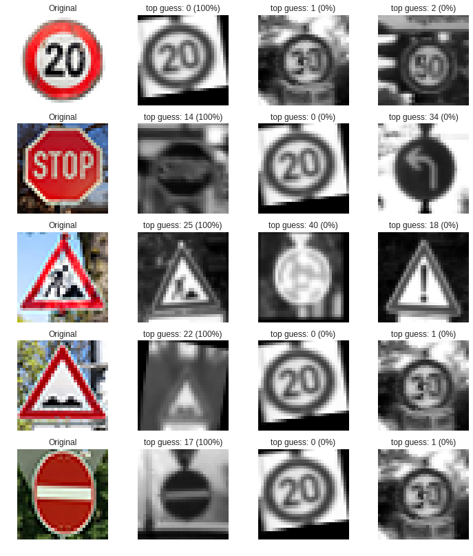
16. Finally, I Output Top 5 Softmax Probabilities For Each Image Found on the Web

softmax_logits = tf.nn.softmax(logits)
top_k = tf.nn.top_k(softmax_logits, k=3)
with tf.Session() as sess:
    sess.run(tf.global_variables_initializer())
    saver = tf.train.import_meta_graph('./lenet.meta')
    saver.restore(sess, "./lenet")
    my_softmax_logits = sess.run(softmax_logits, feed_dict={x: X_images_test})
    my_top_k = sess.run(top_k, feed_dict={x: X_images_test})    
    fig, axs = plt.subplots(len(images),4, figsize=(12, 14))
    axs = axs.ravel()
    
    for i, image in enumerate(images):
        axs[4*i].axis('off')
        axs[4*i].imshow(image)
        axs[4*i].set_title('Original')
        
        for j in range(3):
          guess = my_top_k[1][i][j]
          index = np.argwhere(y_validation == guess)[0]
          axs[4*i+j+1].axis('off')
          axs[4*i+j+1].imshow(X_validation[index].squeeze(), cmap='gray')
          axs[4*i+j+1].set_title('top guess: {} ({:.0f}%)'.format(guess, 100*my_top_k[0][i][j]))

My final model results were:

• validation set accuracy of 0.987
• test set accuracy of 1

Conclusions

I chose LeNet architecture because, as we see in the course, I it is a great model architecture for classifying images. I wanted to try this one before anything else, and as I found that it has a great performance, in addition to the augmentation techniques, I prefered this solution, simple and solve the problem.

This application will help to a self-driving car to understand, as well as we do, what comes ahead on the road and predict what actions it should have to make given the time.